1.1. Real-Time Animation of Graphs
Real-time graphs are helpful when you need to visualise values from sensors or databases in real-time. This serves an important function in many critical industries where continuous monitoring of data is required, e.g. monitoring ground movement, emission control in tunnel environment, stock market etc.
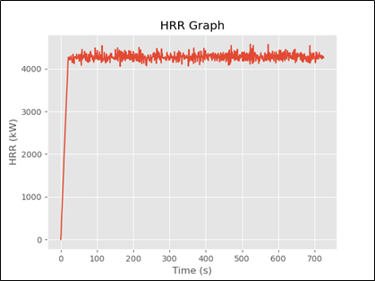
This article goes through the Python code required to visualise the Heat Release Rate (HRR) graph in real-time to verify the simulation is generating the fire size as required. You can use data from any real-time sensors or simulations and follow the steps provided in this article. In this article, I have used the data generated by a CFD software called Fire Dynamics Simulator (FDS) developed by the National Institute of Standards and Technology (NIST).
1.2. Python Packages used in the script
Pandas and Matplotlib are the two Python packages that are required in the script. Pandas is used to load the data whereas, Matplotlib is used to generate and style the graph.
From Matplotlib package ‘Pyplot’ function is required to style the graphs similar to Matlab and from class matplotlib.animation, Funcanimation is required to repeatedly call a function to create an animation. In this script, ‘ggplot’ style is used to style the graph. Different style sheets are available in Matplotlib which can be found here: https://matplotlib.org/stable/gallery/style_sheets/style_sheets_reference.html.
1.3. CSV Data
Data for generating a real-time graph is gathered from the FDS simulation.
In the FDS simulation folder, the HRR data can be found within a CSV file name with an ‘_HRR.csv’ suffix. Data in the first two columns are required to generate the HRR graph. To load the data to Python, we will use the Pandas package as shown in the next section.
Data generated by FDS can be downloaded from my GitHub repository here https://github.com/jabirjamal/jabirjamal.com/tree/main/FE/FE_04.

1.4. Python script
The following block of code is used to load the required Python packages. If you are using Jupyter Notebook use the magic command ‘%matplotlib notebook’ to generate the graph within the notebook. This is not required for any other IDE.
import pandas as pd
import matplotlib.pyplot as plt
plt.style.use(‘ggplot’)
from matplotlib.animation import FuncAnimation
%matplotlib notebook
As mentioned in the previous section, ‘Time’ and ‘HRR’ values are required to generate the HRR graph. These columns in the Pandas DataFrame are assigned to variables x and y as shown in the block of code below. The code also shows you how to use the Pyplot function imported as ‘plt ’ to style the axes labels and title.
These lines of code are grouped within a function called ‘animate’ so it can be called any number of times as required.
Note that we have skipped row 1 (‘units’) and used row 2 (‘parameters’) as the column headings.
def animate(i):
    data = pd.read_csv(r'C:\OneDrive\JabirJamal.com\Fire Engineering\FE_05_RealTime_Graph\FDS\Model1_hrr.csv', skiprows=1)
    x = data['Time'] # assigning 'Time' column to x variable
    y = data['HRR'] # assigning 'HRR' column to y variable

    plt.cla() # clear axis after plotting individual lines
    plt.plot(x, y, label = 'HRR') # selecting the x and y variables to plot
    plt.xlabel('Time (s)') # label x axis
    plt.ylabel('HRR (kW)') # label y axis
    plt.title('HRR Graph')
To generate the graph within the animate function continuously at particular intervals, we can use the function ‘FuncAnimation’. The following arguments are passed to the ‘FuncAnimation’ to generate the animation:
· Plt.gct(): plt.gcf (get current figure) will reload the plat based on the data saved in the ‘data’ DataFrame
· Animate: animate argument will call the function continuously.
· Interval: interval = 2000. The frames will be updated every 2 seconds. The default unit of ‘interval ’ is milliseconds.
· Frames: frames = 200. Generates 200 frames during the simulation to create the animation.
· Repeat: Repeat = False. This will stop the simulations after generating the specified number of ‘frames’.
ani = FuncAnimation(plt.gcf(), animate, interval = 2000, frames = 200, repeat = False)
plt.tight_layout() # adds padding to the graph
plt.show() # show graph
Youtube Video of Animation
Use the following code block (instead of plt.show()) to download the animation as a video.
video = ani.to_html5_video()
html = display.HTML(video)
display.display(html)plt.close()
1.5. Github and Medium
You can find the files used in this article in my GitHub repository here: https://github.com/jabirjamal/jabirjamal.com/tree/main/FE/FE_04
You can follow me on Medium here: https://jabirjamal.medium.com/