Determining sprinkler activation time using Alpert’s correlations

While designing fire safety systems, a fire engineer needs to determine the expected fire size based on the project details. In Australia, Alpert’s correlation and Heskestad equations are typically used to determine the fire size at which a sprinkler head activates.

In this blog, I have written a Python script to calculate the time and fire size at sprinkler activation.

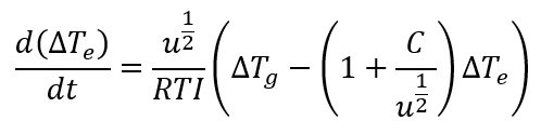
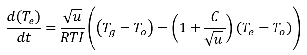
Heskestad equation

This section provides the equation developed to determine the sprinkler response time. Refer to ‘Quantification of thermal responsiveness of automatic sprinklers including conduction effects’ by Gunnar Heskestad and Robert G.Bill, JR, published in Fire Safety Journal, 14 (1988) 113–125

Equation 15:

Where,

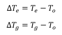
The above equation can be re-written as,

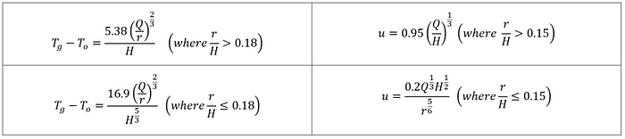
Alpert Equations

This section provides equations related to gas velocity and temperature at the ceiling level with the plume. These equations are published by R.L. Alpert in ‘ Calculation of response time of ceiling-mounted fire detectors ‘.

Where,

Step 1. Import relevant Python packages

import pandas as pd
import plotly.express as px

Step 2. Enter user inputs

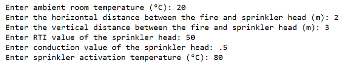
while True:
    try:
        amb_temp = float(input('Enter ambient room temperature (°C): '))
        rad_distance = float(input('Enter the horizontal distance between the fire and sprinkler head (m): '))
        height_above_fire = float(input('Enter the vertical distance between the fire and sprinkler head (m): '))
        RTI = float(input('Enter RTI value of the sprinkler head: '))
        c = float(input('Enter conduction value of the sprinkler head: '))
        activation = float(input('Enter sprinkler activation temperature (°C): ')) 
        break
    except ValueError as e:
        print('Error: Enter a valid number')

Step 3. Select fire growth rate

t_sq_list = ["slow", "medium", "fast", "ultra-fast"]
t_sq  = Nonewhile t_sq not in t_sq_list:
    t_sq = input('Enter fire t² growth rate. Select from the list [slow, medium, fast, ultra-fast]: ').lower().strip()if t_sq == 'slow':
    growth = 0.00293
elif t_sq == 'medium':
    growth = 0.01172
elif t_sq == 'fast':
    growth = 0.0469
else:
    growth = 0.1876
    
print('Fire growth rate coefficient is: ' + str(growth))

Step 4. Create a DataFrame

Step 4.1. Create an empty DataFrame and assign column names

index = pd.RangeIndex(0, 1308, 1) # a slow t² fire will take 1307 seconds to reach 5 MW
columns = ['Time', 'HRR', 'Gas Temp 1', 'Gas Temp 2', 'Gas Vel 1', 'Gas Vel 2', 'Gas Temp', 'Temp Sprinkler']df = pd.DataFrame(index=index, columns=columns)
df = df.fillna(0) # with 0s rather than NaNs
df.head()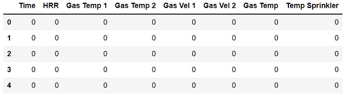

Step 4.2. Populate HRR column

df['Time'] = df.index
df['HRR'] = df['Time']*df['Time']*growth
df.head()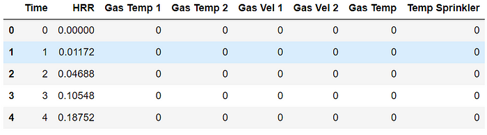

Step 4.3. Determine gas temperature

if rad_distance/height_above_fire > 0.18:
    df['Gas Temp 1'] = (5.38*(df['HRR']/rad_distance)**(2/3))/(height_above_fire)
    df['Gas Temp'] = df['Gas Temp 1'] + amb_temp
    a = 'one'
else:
    df['Gas Temp 2'] = (16.9*(df['HRR'])**(1/3))/height_above_fire**(5/3)
    df['Gas Temp'] = df['Gas Temp 2'] + amb_temp
    a = 'two'df.head()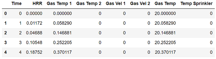

Step 4.4. Determine gas velocity

if rad_distance/height_above_fire <= 0.15:
    df['Gas Vel 1'] = (0.2*df['HRR']**(1/3)*height_above_fire**(1/2))/(rad_distance**(5/6))
    b = 'one'
else:
    df['Gas Vel 2'] = 0.95*((df['HRR']/height_above_fire)**(1/3))
    b= 'two'df.head()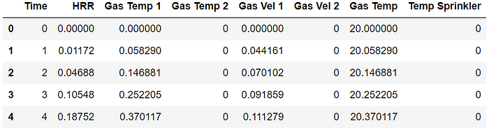

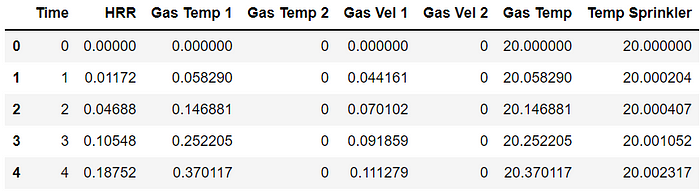
Step 5. Generate the DataFrame

x = 2
# initialise row 0
df.loc[0, 'Temp Sprinkler'] = amb_temp
if (a == 'one') & (b == 'one'):
    # initialise row 1
    df.loc[1, 'Temp Sprinkler'] = amb_temp + ((df.loc[1,'Gas Vel 1']**0.5)/RTI)*((df.loc[1,'Gas Temp']-amb_temp)-((1+(c/df.loc[1,'Gas Vel 1']**0.5)))*(df.loc[0,'Temp Sprinkler']-amb_temp))

    # initialise remaining rows
    while x < 1308:
        df.loc[x,'Temp Sprinkler'] = df.loc[x-1, 'Temp Sprinkler'] + ((df.loc[x-1, 'Gas Vel 1']**0.5)/RTI)*((df.loc[x-1, 'Gas Temp']-amb_temp)-((1+(c/df.loc[x-1, 'Gas Vel 1']**0.5)))*(df.loc[x-1, 'Temp Sprinkler']-amb_temp))  
        x = x+1

elif (a == 'one') & (b == 'two'):
    df.loc[1, 'Temp Sprinkler'] = amb_temp + ((df.loc[1,'Gas Vel 2']**0.5)/RTI)*((df.loc[1,'Gas Temp']-amb_temp)-((1+(c/df.loc[1,'Gas Vel 2']**0.5)))*(df.loc[0,'Temp Sprinkler']-amb_temp))

    while x < 1308:
        df.loc[x,'Temp Sprinkler'] = df.loc[x-1, 'Temp Sprinkler'] + ((df.loc[x-1, 'Gas Vel 2']**0.5)/RTI)*((df.loc[x-1, 'Gas Temp']-amb_temp)-((1+(c/df.loc[x-1, 'Gas Vel 2']**0.5)))*(df.loc[x-1, 'Temp Sprinkler']-amb_temp))  
        x = x+1

elif (a == 'two') & (b == 'one'):
    df.loc[1, 'Temp Sprinkler'] = amb_temp + ((df.loc[1,'Gas Vel 1']**0.5)/RTI)*((df.loc[1,'Gas Temp']-amb_temp)-((1+(c/df.loc[1,'Gas Vel 1']**0.5)))*(df.loc[0,'Temp Sprinkler']-amb_temp))

    while x < 1308:
        df.loc[x,'Temp Sprinkler'] = df.loc[x-1, 'Temp Sprinkler'] + ((df.loc[x-1, 'Gas Vel 1']**0.5)/RTI)*((df.loc[x-1, 'Gas Temp']-amb_temp)-((1+(c/df.loc[x-1, 'Gas Vel 1']**0.5)))*(df.loc[x-1, 'Temp Sprinkler']-amb_temp))  
        x = x+1

else:
    df.loc[1, 'Temp Sprinkler'] = amb_temp + ((df.loc[1,'Gas Vel 2']**0.5)/RTI)*((df.loc[1,'Gas Temp']-amb_temp)-((1+(c/df.loc[1,'Gas Vel 2']**0.5)))*(df.loc[0,'Temp Sprinkler']-amb_temp))

    while x < 1308:
        df.loc[x,'Temp Sprinkler'] = df.loc[x-1, 'Temp Sprinkler'] + ((df.loc[x-1, 'Gas Vel 2']**0.5)/RTI)*((df.loc[x-1, 'Gas Temp']-amb_temp)-((1+(c/df.loc[x-1, 'Gas Vel 2']**0.5)))*(df.loc[x-1, 'Temp Sprinkler']-amb_temp))  
        x = x+1

df.head()

Step 6. Plot the graph

Step 6.1. Determine the sprinkler activation temperature

try:
    act_time = df.loc[df['Temp Sprinkler']>activation, 'Time'].iloc[0]
except:
    print('The sprinkler does not activate')

Step 6.2. Determine the HRR at sprinkler activation

try:
    act_hrr = round(df.loc[df['Temp Sprinkler'] > activation, 'HRR'].iloc[0],1)
except:
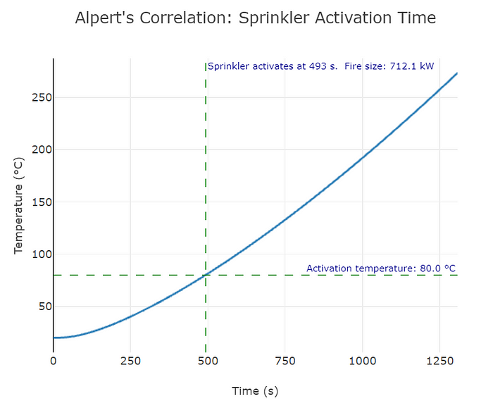
    print('The sprinkler does not activate')

Step 6.3. Create annotation for horizontal and vertical lines

act_time_text = 'Sprinkler activates at ' + str(act_time) + ' s.' + '\n'+ ' Fire size: ' + str(act_hrr) + ' kW'

act_temp_text = 'Activation temperature: ' + str(activation) + ' °C'

Step 6.4. Generate the graph

fig = px.line(df, x="Time", y="Temp Sprinkler", title="Alpert's Correlation: Sprinkler Activation Time", template = 'none')
fig.update_layout(
    autosize=False,
    width=600,
    height=500,
    yaxis=dict(
       title_text="Temperature (°C)",
        titlefont=dict(size=12),
    ),
    xaxis=dict(
       title_text="Time (s)",
        titlefont=dict(size=12),
    )
)
fig.update_layout(
    title={
        'y':0.9,
        'x':0.5,
        'xanchor': 'center',
        'yanchor': 'top'})
fig.update_layout(
    xaxis = dict(
        tickmode = 'linear',
        tick0 = 0,
        dtick = 250
    )
)

fig.add_hline(y=activation, line_width=1, line_dash="dash", line_color="green", annotation_text = act_temp_text)
fig.add_vline(x=act_time, line_width=1, line_dash="dash", line_color="green",  annotation_text = act_time_text)

fig.update_annotations(font_size=10, font_color = 'darkblue')
fig.show()